| 12.3. Semi-Automated TMA generation | ||
|---|---|---|
 | Chapter 12. Management of TMA and TUA solutions |  |
| 12.3. Semi-Automated TMA generation | ||
|---|---|---|
| | Chapter 12. Management of TMA and TUA solutions | |
Many Debrief users have high-performance workstations that have sufficient processing power to produce an initial best-guess at a solution for target tracks based on bearing data. In 2012 talks started regarding the delivery of such a capability to analyst usesrs. Significantly, it was perceived that an automated approach would benefit from multi-leg engagements, engagements that are typically challenging using the existing Debrief manual TMA capabilities.
Following exploratory discussions with Atlas Elektronik UK regarding the FRITMA tool it was determined by the relevant stakeholders that a custom-built TMA algortihm would be a viable solution for the requirement. This new Debrief feature was to be called Semi Automatic Track Construction (SATC)
![[Note]](images/note.gif) | Note |
|---|---|
|
Further detail regarding the strategies and algorithms used in SATC are found later in this document, in Chapter 20, Semi Automated Track Construction (SATC) |
The concept of Bearings Only Target Motion Analysis, or Bearings Only Tracking (BOT) is an established field of mathematics. An easy intro to this is covered in this users online guidance for the 688i game. This system utilises a variant on that concept. Whilst BOT focuses on the production of a near-real time estimate of the current state (location, course, speed) of the subject vehicle, this system performs the process time-late, aiming to produce a whole segment of vehicle track. The time-late nature of the undertaking (possibly several weeks later) means that an analyst has the opportunity to research other information about the vehicle track to contribute to the algorithm. This other information may be through acoustic analysis, supplementary documentation, or third-party sensors.
A set of parameters that any target solution must meet - for example an analyst may know the range of speeds of a class of vessel sufficient to say "any solution track for this vessel must be within 2 and 9 knots".
A subjective contribution from an analyst, such as "I believe the vessel is travelling at 4 knots". The SATC will consider values other than the estimate, but solutions that match the estimate will be favoured.
A piece of information that is used in development of target solutions. This may be a measurement (such as range, bearing or frequency) data, an analyst forecast (a prediction, such as speed range), or one of a hidden set of analysis contributions that deduce further constraints based on other contributions.
The collection of information and knowledge that is used to produced target solutions
A period of time for which it is known that the target vessel is either on steady course/speed (Straight Leg) or is manoeuvring (Altering Leg)
An indication of the level of fidelity to be considered by the SATC algorithm. For the LOW, MEDIUM, HIGH precisions the algorithm is allowed to run for 5, 15 and 30 seconds resp. For these precisions, the number of solutions considered for each processing cycle are 45, 70 and 120 resp.
A single permutation of target track, comprised of a series of legs - both altering and straight.
A series of meetings with Dr Iain McKenna (BAE Systems) led to a strategy where informed analysts would be able to submit a series of contributions representing knowlege they held regarding a vessel engagement. This flow of knowledge and interaction with the algorithm is as recorded below
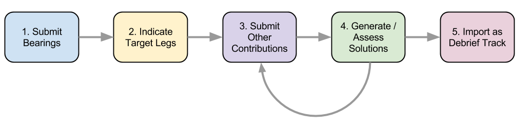
SATC Sequence
Bearing data lies at the core of the SATC algorthm, proving one of the most useful constraints on potential target track. The solution generation process is started by submitting a block of bearings to a solution.
The second-most important contribution is the knowledge of time periods where the target is believed to be travelling in a straight line. Again, this greatly reduces the number of candidate solutions that need to be considered.
Once the first two contributions are in place, the analyst is then able to submit his knowledge/hypotheses regarding target course, speed, or the range to the target. These forecasts can relate to the whole target solution, particular legs, or even discrete periods of time between those legs.
The analyst can then trigger the generation of a solution. The solution is optimal in regard to the contributions that the analyst has submitted. If the solution does't match the analysts expectation, or if it just doesn't look right, then the analyst can submit further contributions, as appropriate.
Ultimately, if/when the analyst is happy with the solution produced he can import the solution into Debrief, either as a collection of legs (to be used in the existing manual TMA process), or directly as a conventional Debrief track.
Internally, the SATC process runs in two stages. The first considers hard-constraints that the analyst has recorded for the engagement. These constraints are intelligently fused into a consolidated body of constraints, one set for each potential target location (one location is produced for each bearing measurement). This phase is able to run very quickly, since it just deals with hard facts. It is possible to view the set of constraints changing live on the Debrief plot whilst the hard-constraints are manipulated.
The second stage is where candidate solutions are produced. This stage can be quite time-consuming, so it is only run on analyst request. The stage produces an imaginary grid over the potential start and end positions for each straight leg. The algortihm then looks at the possible straight courses between combinations of these points. An optimisation algorithm reduces the number of permutations that need to be considered. The optimisation algorithm also discards solutions that, whilst mathematically optimal, do not represent achievable successive courses (due to simple speed/time calculations).
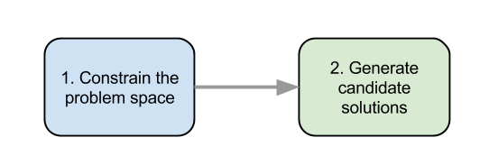
SATC Process
The following screenshot shows a TMA scenario using simulated data. The ownship track is shown in Blue, the truth target track is shown in Red, and the generated solution is shown in Yellow. The range error between truth and generated track is shown in the Range vs Time Plot at the foot of the image. The scenario is particularly challenging, given that there are more target manoeuvres than ownship manoeuvres, the target is quite distant, and the bearing rates are relatively low.
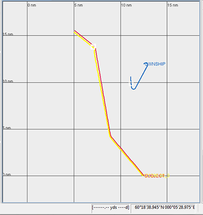
Sample solution
SATC scenarios are managed from within the Maintain Contributions view within Debrief. This view opens automatically when a new scenario is created.
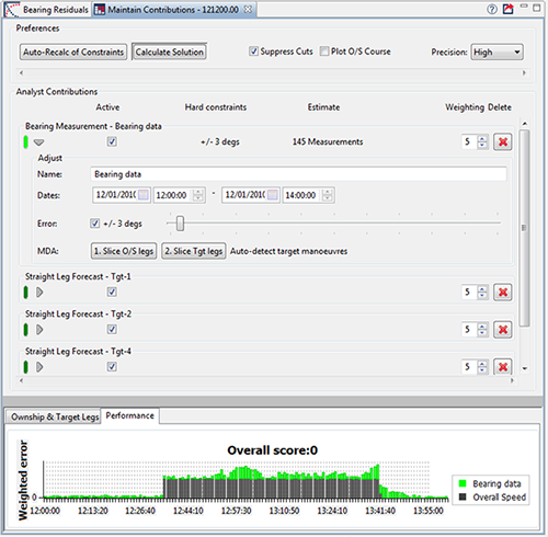
Maintain Contributions View
The following sections describe the three parts of the Maintain Contributions View
Preferences. This panel provides overall control of the scenario.
This toggle button tells SATC whether it should recalculate the constraints each time a contribution is changed
Actually calculating the solution can take up to several minutes, so the overall solution is only calculated when this button is pressed
Whether to allow Debrief to Suppress the least significant cuts. Greater precision settings allow suppression of fewer cuts.
Used to indicate which of the three precision levels are required in solution generation.
Analyst Contributions. This contains a list of the contributions provided by the analyst. For each contribution, this data is present:
Each contribution is presented inside it's own screen object. The contribution name is provided at the top-left of this block
Some contributions have hard constraints. In the earlier screenshot you can see that the Speed Forecast has hard constraints of 5-15 knots. No solution will go outside these bounds.
Where an estimate is provided, it is shown here. For the Speed Forecast in the earlier screenshot, you can see that an estimate of 13 knots has been provided. So, solutions will be favoured if they have a target speed nearer to 13 knots.
The weighting is a way of the analyst tuning the TMA process. Higher weightings figure more strongly in the generated solutions.
Use this to delete a contribution. It will also disappear from the Layer Manager.
Performance. The performance graph is an indication of progress of the SATC algorithm, as a series of states along the whole solution. For each timed state object the graph shows one or more bars. A bar is shown for each contribution that is capable of calculating solution error - with some error scores shown per state (such as for Bearing Measurement Contribution) or an error shown for a whole leg (such as for an estimated leg speed). The error shown is normalised to a zero-one value within the allowable min/max range (or bearing error for bearing data), then scaled according to the weighting value for that contribution.
Analysis support. In the toolbar for the Maintain Contributions view is a button to export a summary of the scenario to the clipboard in CSV format. This format includes a series of x,y, date-time, course, speed ownship state measurements, followed by a series of time-stamped bearings. The X/Y and date-time have been made relative to an arbitrary location to hide any potentially sensitive data. Access to the data eases the task of externally analysing the scenario.
| |  | |
| 12.2. TMA Management |  | Chapter 13. Support for DIS Protocol |